Deep Learning Model Compression (ii)

We need model compression because of many edge devices having limited computational power and capability. IoT devices usually runs under very restrictive power constraints due to limitations on either power source or heat dissapation. With the low cost nature of these devices, their computational capabilities are also usually limited (e.g. lack of FPU or SIMD) and this can worsen the power constraint problem we already had in edge neural network inferencing.

Many IoT devices are powered by batteries, and requires them to run over long period of time. Several well-developed technology for IoT devices under this type of constrainsts (such as LoRa) relies on intermediant shutdown of devices. However this approach are not very suitable for edge inferencing. E.g. a low frame rate recurrent object detection model requires 1s+ to initialize and have the device in deep sleep until waked up by sensors is not usually an option. If we keep the model running, and sustain the battery for a long time, we need compressed, smaller model to run it under a lower processor frequency (as power usually scales at the square of frequency, or computational power under same instruction per clock).

Chip cost is also a big factor limiting IoT devices’ capability of running large, uncompressed neural network. Chip cost limits the chip size, lithography technology node (and in turn power efficienty) and IP cores it can use. For example, large cache on chips are very expensive to produce as they cost a lot of die areas, and smaller cache we see on IoT devices makes running larger models exponentially inefficient due to cache misses when running the network. Using older lithography technology node in low cost IoT chip manufacturing is also a limiting factor to its power constraint due to lack of efficiency associated with older lithography nodes. IP core license fees also comes into play in limiting the capabilities of low cost IoT devices running large and uncompressed neural network. The FPUs built-in may be inefficient in running fp32 operations, or it might not have an FPU at all (and soft float is very inefficient), so it will require model to be converted from e.g. fp32 when native to training to e.g. int8 for edge inferencing.

Given the above reasons, I illustrate the importance of model compression. Besides Pruning and Quantization, low-rank approximation and knowledge distillation are othe two well-known methods.

Low-Rank Approximation

It is an effective model compression technique to not only reduce parameter storage requirement, but to also reduce computations.

So far, low-rank approximation has been successfully applied to speech recognition and language models.

SVD stands for Singular-value decomposition, and it is a matrix factorization. SVD is a popular low-rank approximation approach generally applied to the weights of fully connected layers where compact storage is achieved by keeping only the most prominent components of the decomposed matrices. It has several advantages, such as reducing training time.

Low-rank Matrix Decomposition(Source)

I will use an example to explain how matrix factorization reduces runtime

say we have a matrix Y
Y = W x X where W = M x K and X = K x 1
so the runtime is M x K

After matrix factorization

Y = W x X = (U x V) x X where U = M x R and V = R x K and X = K x 1
U x (V x X) runtime is R x K + M x R = R x (M+K)

To compare two total runtime

R x (M+K) < M x K

So here I demonstrate how the matrix factorization helps in reducing training time.

SVD, Tucker decomposition and CP(Canonical Polyadic) decomposition are the most well-known low-rank approximation methods, however, they would result in lowering model accuracy because decomposed layers hinder training convergence.

According to Learning Low-Rank Approximation for CNNs, Lee et al. propose a new training technique that finds a flat minimum in the view of low-rank approximation without a decomposed structure during training.

Fig1 (source)

Figure 1 shows the DeepTwist optimization procedure for low-rank approximation.

At each weight distortion step, parameter tensors are decomposed into multiple tensors following low-rank approximation, which means effectively injecting noise into parameter tensors without modifying the structure

DeepTwist has two advantages compared with previous methods. This first is noise is added only when a set of parameters is close to a local minimum to avoid unnecessary escapes. The second is escape distance is determined by noise induced by low-rank approximation

Training loss and Test accuracy comparison on ResNet-32 using CIFAR-10 (source)

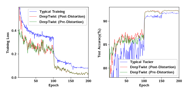
In this figure, it shows compared to typical training, DeepTwist improves training loss and test accuracy throughout the entire training proces.

Initially, the gap of training loss and test accuracy between pre-distortion and post-distortion is large. Such a gap,however, is quickly reduced through training epochs, because a local minimum found by DeepTwistexhibits a flat loss surface in view of low-rank approximation.

Knowledge Distillation

Knowledge Distillation in introduced by Hinton et al, it is the general solution of previous technique proposed by Caruana, which is to minimize the logits space/ or we could call it output layer using RMSE.

Transfer the knowledge from a cubersome teacher model to small model.

The setup of training process of the student(Source)

Neural networks typically produce class probabilities by using a “softmax” output layer that convertsthe logit, zi, computed for each class into a probability, qi, by comparingziwith the other logits.

Use the class probabilities produced by the cumbersome model as “soft targets” for training the small model.

Q_i corresponds to the value of neuron i in the i layer
The value of T=1 corresponds to regular softmax behavior.

Simplest form of distillation:

1. Train the cumbersome model using a temperature of 1
2. Train the distilled model with a high temperature in its softmax

Train the Distilled model using two objective functions to modify the soft target:

1. cross entropy with the soft target
2. cross entropy with the correct labels

The first loss term uses the soft labels & soft predictions

The second loss term uses hard prediction and hard labels.

source

The authors conducted their experiments on MNIST and Voice Recognition problems and obtained excellent results

Additional resources for understanding the methods

Here I also find an open-source implementation of the paper —

karanchahal/distiller

References:

SVD and Data Compression Using Low-rank Matrix Approximation

Knowledge Distillation

1. https://dl.acm.org/doi/pdf/10.1145/3290420.3290444
2. https://www.mathworks.com/company/newsletters/articles/what-is-int8-quantization-and-why-is-it-popular-for-deep-neural-networks.html
3. https://electronics.stackexchange.com/questions/64381/power-consumption-and-frequency
4. https://arxiv.org/pdf/1503.02531.pdf
5. https://arxiv.org/pdf/1905.10145.pdf